PSYC4411

Learning Representations

Neural Networks as Psychological Tools

Week 9 · Semester 1, 2026

Today’s Plan

Perceptrons and multi-layer networks — what they look like
Activation functions — where the magic happens
How neural networks learn — forward pass, loss, backprop
Training in practice — epochs, batches, and validation
Overfitting in neural networks — when power becomes a problem
When to use NNs (and when not to)
NNs in psychology — real applications
Getting ready for Week 10 — PyTorch and complex debugging

What Is a Neural Network?

Starting with something you already know

The Perceptron: You Already Know This

Remember logistic regression from Week 5?

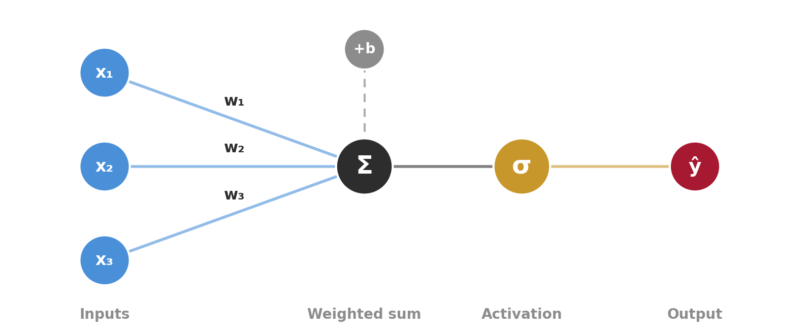
A single perceptron is logistic regression. Multiply inputs by weights, add a bias, apply sigmoid. That’s it. A neural network is just many of these stacked together.

The Connection to What You Know

Logistic Regression (Week 5)

Multiply each feature by a weight

Add them up (plus a bias term)

Apply the sigmoid function

Get a probability between 0 and 1

Perceptron (1958)

Multiply each input by a weight

Add them up (plus a bias term)

Apply an activation function

Get an output

These are the same computation described in different vocabularies. The perceptron was invented by psychologist Frank Rosenblatt in 1958 — inspired by how neurons in the brain combine signals.

Multi-Layer Perceptrons (MLPs)

Stack multiple layers of perceptrons together:

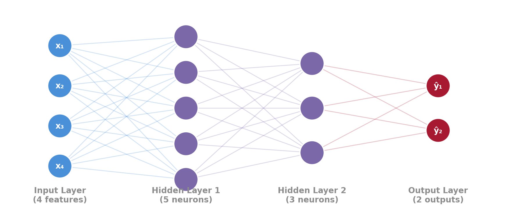
Why Layers Matter: Universal Approximation

A single perceptron can only learn straight-line boundaries (like logistic regression)
Add a hidden layer → the network can learn curves
Add more neurons/layers → it can learn any pattern, no matter how complex

Universal approximation theorem: A neural network with just one hidden layer (and enough neurons) can approximate any mathematical function. In theory, it can learn anything.

“Can learn anything” sounds great — but it also means neural networks can learn noise just as eagerly as signal. This is why overfitting is the central challenge.

Think About It

These models were inspired by neurons in the brain — but they don’t actually work like brains. Real neurons are vastly more complex.

Is calling these “neural networks” helpful? Does the brain analogy make them easier to understand — or does it create dangerous misconceptions about what AI can do?

Activation Functions

Where non-linearity enters the picture

Two Activation Functions You Need to Know

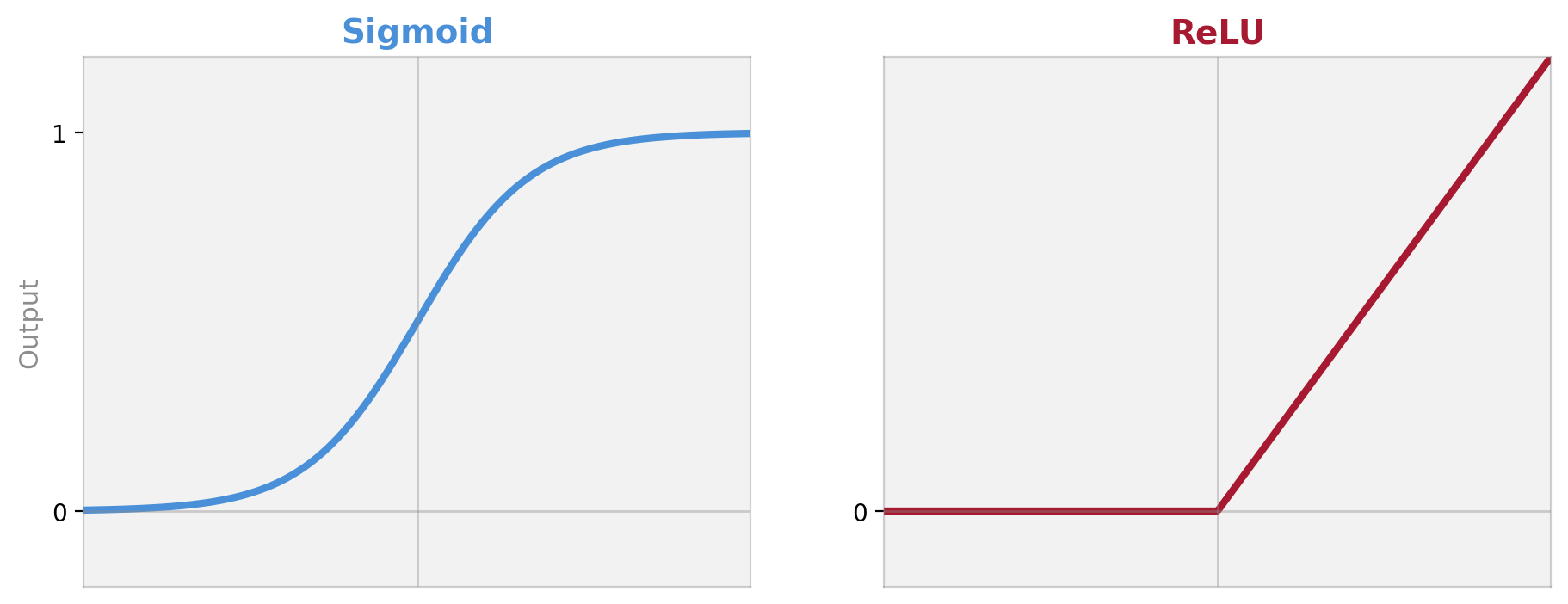
Sigmoid — squashes everything to 0–1. You used this in logistic regression.

ReLU — if negative, output 0. If positive, pass through. The workhorse of modern deep learning.

Why Non-Linearity Matters

Without activation functions: Stacking 100 layers of linear math still gives you… a linear model. No matter how many layers, it collapses to one big multiply-and-add. You’d just get fancy regression.

With activation functions: Each layer can bend the space. The network can learn curved boundaries, complex interactions, and patterns that no straight line could capture.

Analogy: Activation functions are like joints in a robotic arm. Without them, the arm is a rigid stick (linear). With them, it can reach anywhere (non-linear). More joints = more flexibility.

How Neural Networks Learn

Forward, measure, backward, update

The Learning Loop

Forward Pass

→

Compute Loss

→

Backward Pass

→

Update Weights

Forward pass: data flows through the network, producing a prediction
Loss: measure how wrong the prediction is (e.g., MSE, cross-entropy)

Backward pass: figure out which weights contributed most to the error
Update: nudge each weight to reduce the error next time

This cycle repeats thousands of times. Each repetition makes the predictions slightly better.

Gradient Descent: Finding the Bottom

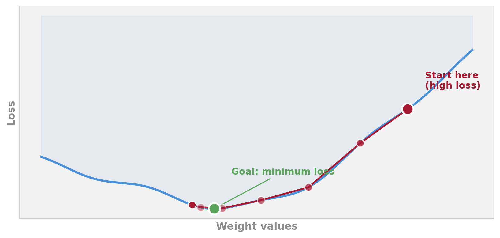
Analogy: You’re standing on a misty hillside and can’t see the valley below. You can only feel the slope under your feet. Gradient descent = always step downhill. Eventually you reach the bottom — or at least a dip.

Learning Rate: How Big Are Your Steps?

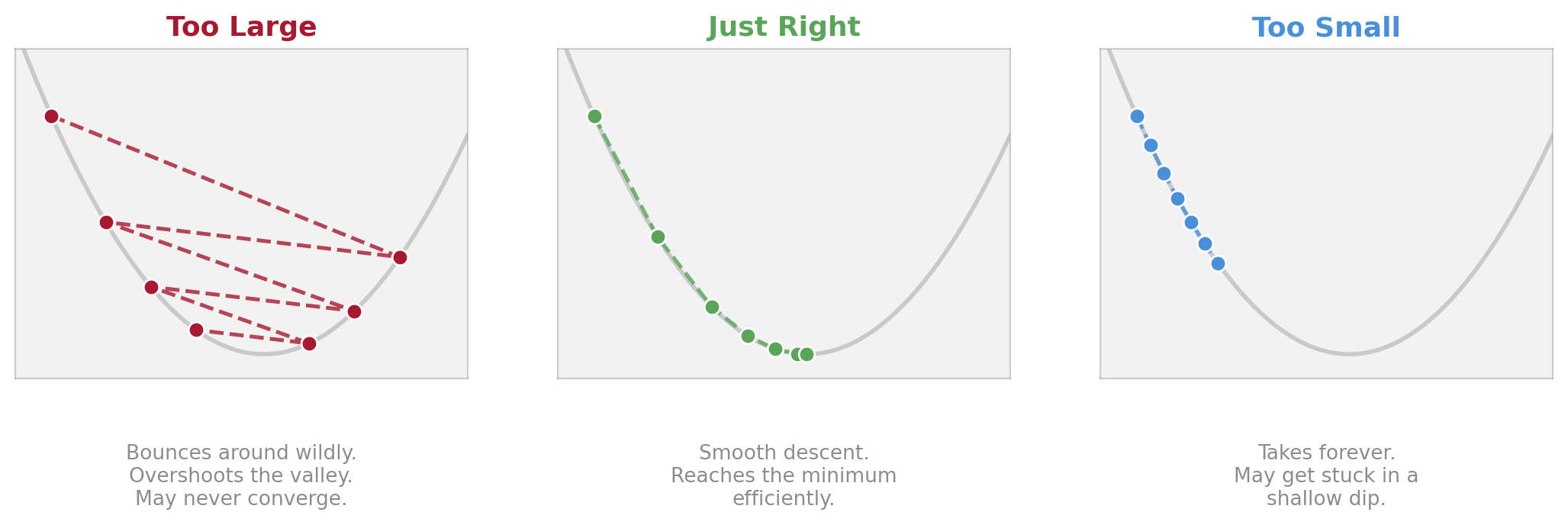
Learning rate comparison: too large, just right, too small

The learning rate is one of the most important settings in neural network training. Getting it right is more art than science.

Think About It

You build a neural network to predict depression severity from lifestyle factors. It achieves 78% accuracy. Your logistic regression from Week 5 achieved 74% accuracy on the same data.

Is the 4% improvement worth the extra complexity? What else would you want to know before choosing one model over the other?

Training in Practice

Epochs, batches, and validation

Key Training Concepts

Epoch

One full pass through the entire training dataset.

Training typically runs for 10–100+ epochs. Like re-reading a textbook multiple times.

Batch

A small chunk of data processed at once (e.g., 32 participants).

Instead of learning from all 3,000 rows at once, update weights after every 32. Faster and often better.

Learning Rate

How much to adjust weights at each step.

Too large = unstable. Too small = slow. Typical starting point: 0.001.

The Training Loop, as a Picture

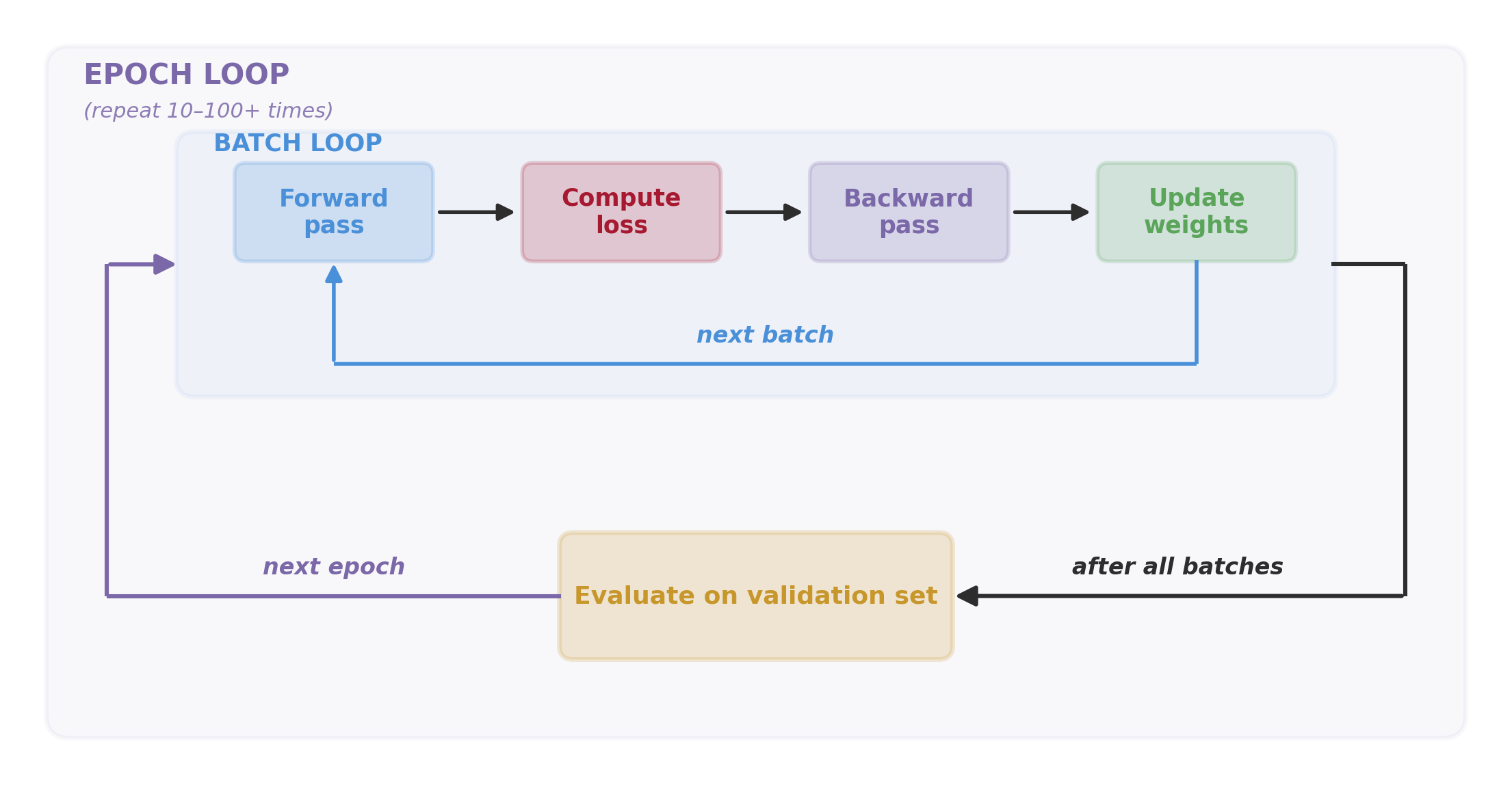
Training loop flow chart: outer epoch loop, inner batch loop with Forward → Loss → Backward → Update, and validation step after each epoch

Two nested loops: the inner batch loop updates weights; the outer epoch loop repeats it many times, checking validation between epochs.

A Training Loop in Plain English

# This is what happens inside model training

for epoch in range(50): # re-read the textbook 50 times

for batch in training_data: # process 32 participants at a time

predictions = model(batch)         # forward pass: make predictions
error = loss(predictions, actual) # how wrong were we?
gradients = backward(error)        # find which weights caused the error
update_weights(gradients)          # nudge weights to reduce error

# After each epoch, check validation set
val_loss = evaluate(model, val_data)
print(f"Epoch {epoch}: val_loss = {val_loss}")

This is what PyTorch does under the hood. In Week 10, you’ll write code that looks very similar to this.

Watching Training Progress

Plot the loss after each epoch — separately for training and validation data:

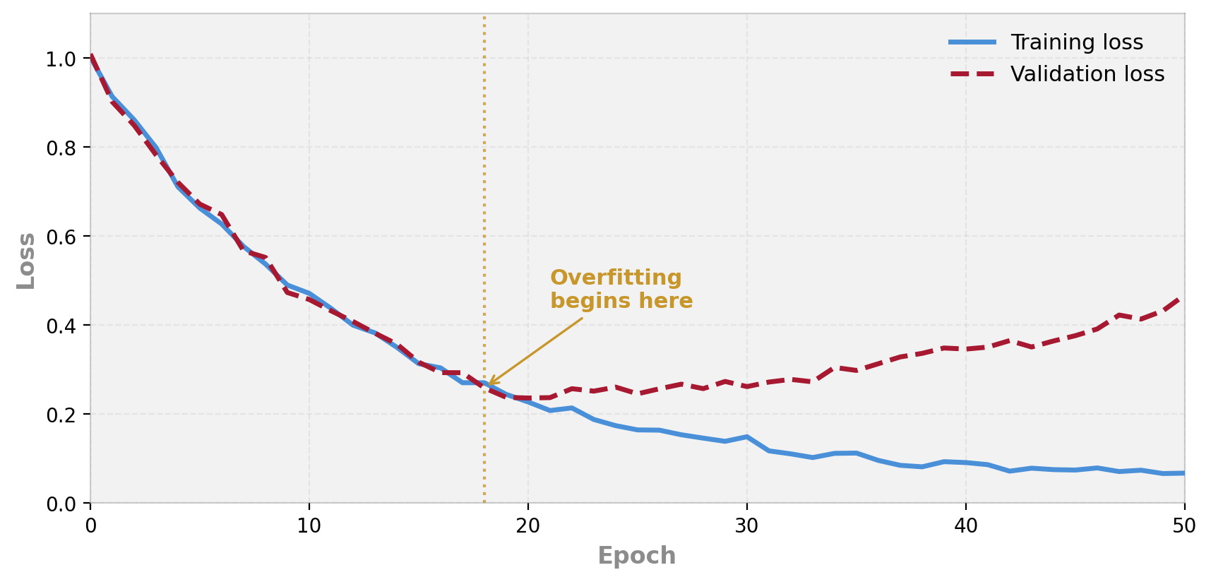
Training and validation loss curves with overfitting

When training loss keeps dropping but validation loss starts rising, the model is memorising the training data instead of learning general patterns. This is the moment to stop.

Overfitting in Neural Networks

When too much power becomes a problem

Why Neural Networks Overfit So Easily

Remember: NNs can learn any pattern, including noise
A typical NN has thousands of weights to adjust (parameters)
With 200 participants and 5,000 parameters, there’s more than enough capacity to memorise every person
This is the same bias-variance tradeoff from Week 3 — but amplified

Week 3 callback: Ridge and Lasso used regularisation to keep linear models honest. Neural networks need their own version of regularisation.

Dropout: Randomly Switching Off Neurons

During each training step, randomly “turn off” some neurons (typically 20–50%).

Forces the network to not rely on any single neuron
Like studying for an exam where any topic might be removed — you learn everything more broadly
At test time, all neurons are active (no dropout)

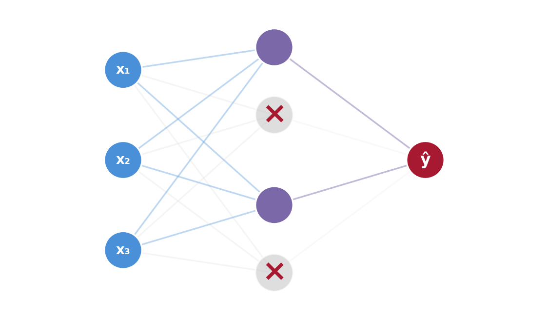
Dropout: some hidden neurons disabled this step

Grey crossed-out neurons are “dropped” this step

Three Defences Against Overfitting

Early Stopping

Stop training when validation loss starts rising.

The simplest and often most effective defence. “Quit while you’re ahead.”

Dropout

Randomly deactivate neurons during training.

Forces distributed learning. Typical rate: 20–50% of hidden neurons dropped per step.

Weight Decay

Penalise large weights (like Ridge regression from Week 3!).

Keeps the model simpler. Same idea as regularisation, applied to neural networks.

In practice, you’ll often use all three together. The tools are different from Week 3, but the principle is identical: constrain the model to generalise.

When to Use Neural Networks

A decision framework

The Decision Framework

NNs Shine When…

Large datasets (thousands+ of observations)

High-dimensional inputs (images, EEG, fMRI, audio, text)

Complex non-linear patterns

You care about prediction accuracy more than interpretability

Traditional ML Wins When…

Small datasets (< 500 participants)

Tabular data (rows and columns, like a spreadsheet)

You need to explain the model (which features drive predictions)

A simpler model performs almost as well

The Honest Truth About Neural Networks

For typical psychology datasets — a few hundred participants, 10–50 survey items, tabular data — a well-tuned Random Forest or Ridge Regression will often match or beat a neural network.

NNs need more data to avoid overfitting
NNs need more tuning (architecture, learning rate, epochs, dropout…)
NNs are harder to interpret
NNs are computationally more expensive

Rule of thumb: Try the simplest model first. If it works well enough, stop there. Use neural networks when you have the data, the complexity, and the reason to justify them.

Think About It

A colleague says: “We have 200 participants who completed a 30-item questionnaire. I want to use a deep neural network to predict their therapy outcomes.”

What would you advise? What kind of model would you suggest instead, and why?

Where NNs Transform Psychology

Brain-Computer Interfaces

Decode motor intentions from EEG signals. Enable paralysed patients to control devices with thought alone. Week 10 preview!

Neuroimaging (fMRI)

Classify mental states from brain scans. Detect patterns of neural activity associated with specific cognitive tasks or clinical conditions.

Connectionist Models

Simulate cognitive processes: language acquisition, reading, memory retrieval. NNs as theories of how the mind works — not just prediction tools.

Digital Phenotyping

Predict mental health episodes from smartphone sensor data: movement patterns, typing speed, social media use, sleep–wake cycles.

Think About It

A brain-computer interface uses a neural network to decode movement intentions from EEG. It’s 92% accurate.

Should it be used to control a prosthetic limb? What level of accuracy would you need before you’d trust it for medical use? What about for typing on a screen?

Does the acceptable error rate depend on the consequences of a mistake?

Common Misconceptions

Myth #1

“Neural networks work like brains.”

Reality: They share the metaphor of connected processing units, but biological neurons are vastly more complex. Real neurons use timing, chemistry, and structural changes that artificial neurons don’t capture. The name is historical, not descriptive.

Myth #2

“More layers = better model.”

Reality: Deeper networks are harder to train, need more data, and are more prone to overfitting. For most psychology datasets, 1–3 hidden layers is plenty. Depth without data is a recipe for noise-fitting.

Myth #3

“Neural networks are always better than traditional ML.”

Reality: On tabular data with modest sample sizes, gradient-boosted trees (like XGBoost) and even linear models often outperform neural networks. NNs dominate for images, text, and audio — not spreadsheets.

Two More to Watch For

Myth #4

“Neural networks are black boxes — you can never understand them.”

Partial truth: NNs are harder to interpret than linear models, but techniques exist: feature importance, saliency maps, attention weights. The field of explainable AI (XAI) is growing rapidly. “Hard to explain” is not the same as “impossible to explain.”

Myth #5

“You need a GPU and huge computing power.”

Reality: For the scale of data typical in psychology (hundreds to tens of thousands of rows, not millions), a laptop CPU is fine. You only need GPUs for large-scale image/text models or very deep architectures.

The Big Idea: Learning Representations

Every model you’ve built so far worked with features you chose — sleep hours, DASS items, big-five traits.

Neural networks are different. Each hidden layer learns its own representation of the data — a new way of describing each person, image, or signal. The network discovers what to pay attention to.

Early layers

Capture simple patterns — e.g. “high on items 3, 7, 12”.

Later layers

Combine those into higher-level concepts — e.g. “anxious + sleep-deprived + isolated”.

This is the same idea behind word embeddings and large language models — we’ll come back to it in Week 11.

Week 10: Your First Neural Network in PyTorch

PyTorch — the library we’ll use; already installed in psyc4411-env
New data type: tensors (like NumPy arrays, designed for NNs)
Same workflow: notebook + script, plan-first approach

Quick setup check before next week:

python -c "import torch; print(torch.__version__)"

# A neural network in PyTorch
import torch
import torch.nn as nn

model = nn.Sequential(

nn.Linear(11, 64),   # 11 features → 64 hidden
nn.ReLU(),            # activation function
nn.Dropout(0.3),      # regularisation
nn.Linear(64, 1),    # 64 hidden → 1 output

)

A complete neural network in 7 lines.

New LLM Skill: Complex Debugging

Neural network errors are often silent — the code runs, but the model doesn’t learn. This requires a different debugging approach.

Weak prompt

“My neural network isn’t working. Here’s my code.”

Strong prompt

“My PyTorch model trains for 50 epochs but validation loss stays at 0.69 (chance level for binary classification). Training loss drops to 0.02. Architecture: 11 → 64 → ReLU → 1. Learning rate 0.001. Batch size 32. Here’s my training loop and loss plot. What could cause the val loss to plateau?”

The key difference: share the behaviour (loss values, plots, what you expected vs. what happened), not just the code. Silent bugs need diagnostic context.

LLM Skills Progression

Week	Skill	Core idea
2	Prompting	Give the AI enough context to write good code
4	Debugging	Share the full error context, not just the message
6	Refactoring	Make working code cleaner and more readable
8	Documentation	Write clear methods descriptions for your analysis
10	Complex Debugging	Diagnose silent failures using behaviour, not just errors

Each skill builds on the last. By Week 10, you can prompt, debug, refactor, document, and diagnose silent model failures.

Questions?

PSYC4411 · Week 9

Week 10: Building your first neural network in PyTorch

See you next week