Today's Plan
- From regression to classification — the conceptual shift
- Logistic regression — probabilities, not just labels
- The confusion matrix — four types of prediction
- Classification metrics — beyond accuracy
- Decision thresholds — 0.5 is a choice, not a law
- Decision trees and random forests — interpretable models
- Fairness and ethics — when algorithms affect people
- Getting ready for Week 6
From Regression to Classification
Numbers to categories
The Shift: Numbers → Categories
Regression
Predict a number
“Depression score = 14.3”
Metric: How far off? (MAE, R²)
Classification
Predict a category
“Elevated depression: Yes/No”
Metric: Which errors? (more complex)
When you classify people, the type of mistake matters as much as the number of mistakes.
Binary Classification
- Target has exactly two values — typically coded as 0 and 1
- In psychology, this is everywhere:
- Clinical diagnosis: yes / no
- Treatment response: responder / non-responder
- Risk assessment: at-risk / low-risk
- Dropout prediction: stays / leaves
- You already know this from logistic regression in statistics
- The difference: ML focuses on prediction accuracy, not significance testing
Week 6 target: Classify participants as having elevated depression (PHQ-9 ≥ 5) vs minimal symptoms (PHQ-9 < 5) using real COVID-era survey data.
Logistic Regression
Probabilities, not just labels
The Sigmoid Function
Linear regression draws a straight line. Logistic regression fits an S-shaped curve.
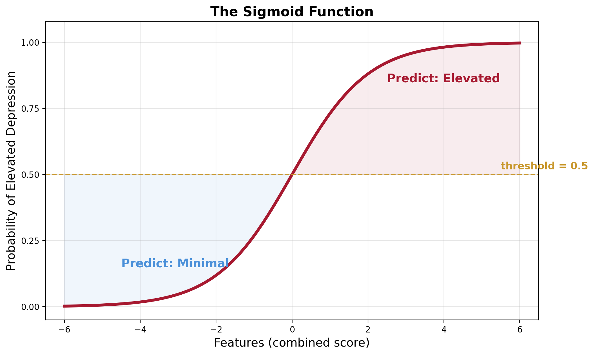
The curve squashes any input to a value between 0 and 1 — we interpret this as a probability.
Probability, Then Decision
- The model outputs: “73% probability of elevated depression”
- Not just “elevated” or “not elevated”
- We choose a decision boundary — typically 0.5
- Above 0.5 → classify as “elevated”
- Below 0.5 → classify as “minimal”
- This threshold is a choice, not a law — more on this soon
The probability output is powerful: it lets us adjust how cautious the model is.
Stats Connection
Logistic regression has been a workhorse of behavioural research for decades.
In Statistics
- “Is this predictor significant?”
- Focus on p-values, odds ratios
- Explain relationships
In ML
- “Can the model correctly identify who belongs to each group?”
- Focus on accuracy, precision, recall
- Predict new cases
Same model, different goals. ML asks: “How well does it work on new data?”
The Confusion Matrix
Four types of prediction
The Confusion Matrix
In screening, false negatives are usually the more dangerous error — we miss someone who needs help.
What This Looks Like in Code
Here's a real confusion matrix from Python — this is what you'll produce in Week 6:
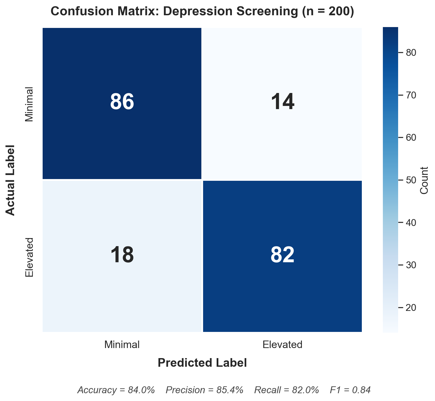
- Top-left (86): Correctly identified as minimal (True Negative)
- Top-right (14): Flagged as elevated but actually minimal (False Positive)
- Bottom-left (18): Missed — actually elevated but predicted minimal (False Negative)
- Bottom-right (82): Correctly identified as elevated (True Positive)
18 missed cases — people with elevated depression that the model didn't catch. Are you comfortable with that?
Classification Metrics
Beyond accuracy
The Accuracy Trap
Accuracy = proportion of predictions that were correct. Seems like the obvious metric.
The trap: Imagine 95% of your sample does not have elevated depression. A model that predicts “not elevated” for everyone achieves 95% accuracy — without learning anything.
- This is the majority-class baseline — always guess the more common class
- Any model must beat this to prove it's actually learning
- Our Week 6 data is nearly balanced (54.5% elevated) — so baseline accuracy ≈ 54.5%
Class imbalance makes accuracy even more misleading — when classes are skewed, always report F1 or AUC alongside accuracy.
The Core Metrics
Precision
Of everyone flagged as elevated, how many actually were?
High precision = few false alarms
Recall (Sensitivity)
Of everyone who actually had elevated depression, how many did we catch?
High recall = few missed cases
F1 Score
Harmonic mean of precision and recall — a single number that balances both.
Specificity
Of everyone who was actually minimal, how many did we correctly identify?
The mirror image of recall.
The Precision–Recall Trade-off
High Precision
When you flag someone, you're almost always right
But you might miss people who need help
High Recall
You catch almost everyone who needs help
But you also flag many who are fine
You can't maximise both at once — making the model more aggressive at catching cases inevitably increases false alarms.
ROC Curve and AUC
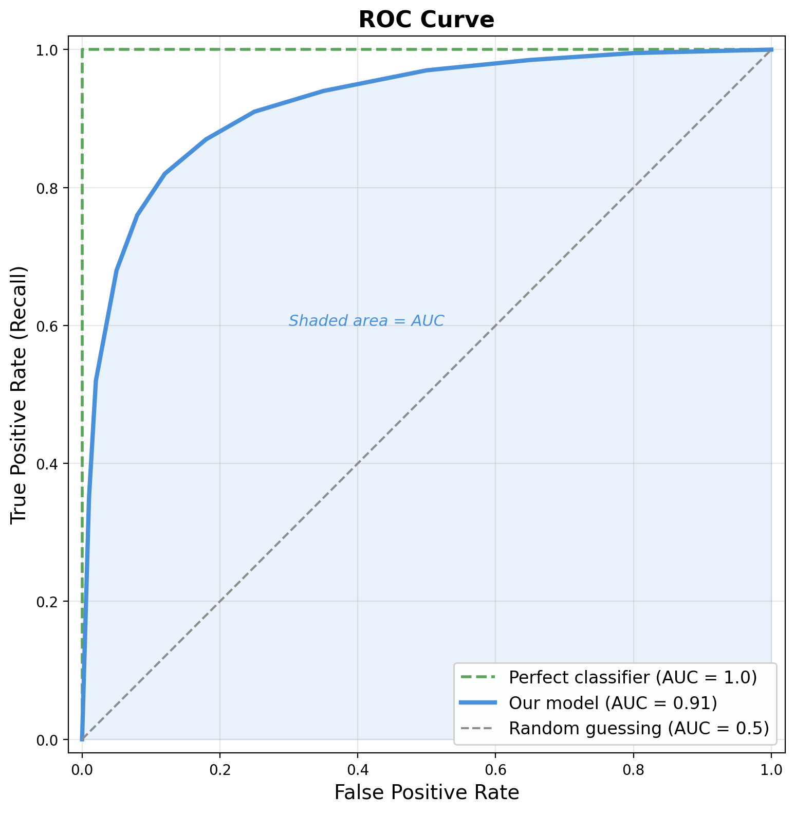
- ROC curve = recall vs false positive rate at every threshold
- AUC = area under that curve
- Perfect model: AUC = 1.0 (green dashed)
- Random guessing: AUC = 0.5 (grey dashed)
- Evaluates the model across all thresholds at once
- Interpretation: “If I pick one elevated and one minimal person at random, how often does the model rank the elevated person higher?”
Decision Thresholds
0.5 is a choice, not a law
The Threshold Is a Choice
Most classifiers output a probability. The threshold for converting that to a label is your decision.
Low (0.3)
Cast a wider net
More true positives
More false alarms
Default (0.5)
Balanced approach
Equal treatment
of both errors
High (0.7)
More conservative
Fewer false alarms
More missed cases
Costs of Different Errors
Screening Programme
Missing someone who needs help is worse than a false alarm.
→ Lower the threshold (e.g., 0.3)
→ Prioritise recall
Clinical Trial Selection
False positives waste expensive resources.
→ Raise the threshold (e.g., 0.7)
→ Prioritise precision
The right threshold depends on the real-world consequences of each type of error.
Decision Trees
If-then rules for prediction
How Decision Trees Work
A decision tree asks a series of yes/no questions about your features, creating a flowchart:

Trees: Strengths and Weaknesses
Strengths
- Interpretable — you can trace exactly why a prediction was made
- Handle non-linear relationships naturally
- No feature scaling needed
- Handle mixed data types
Weaknesses
- Prone to overfitting — unrestricted trees memorise the training data
- Sensitive to small data changes
- Greedy algorithm: locally optimal, not globally
The downside is serious: an unrestricted tree keeps splitting until it perfectly memorises the training data. Like a clinician building an ever-more-elaborate checklist that encodes quirks of specific patients rather than general patterns.
Ensembles & Random Forests
Many trees are better than one
The Ensemble Idea
One tree is interpretable but unstable. What about many trees?
Like asking 100 slightly different experts for their opinion and going with the consensus.

Why Random Forests Work
- Each tree is trained on a random subset of data and features
- Different trees overfit to different quirks
- When you average across many trees, idiosyncratic errors cancel out
- This is the bias–variance trade-off from Week 3:
- Each tree: low bias, high variance
- The ensemble: keeps low bias, dramatically reduces variance
Feature Importance
Random forests rank which features contributed most across all trees:
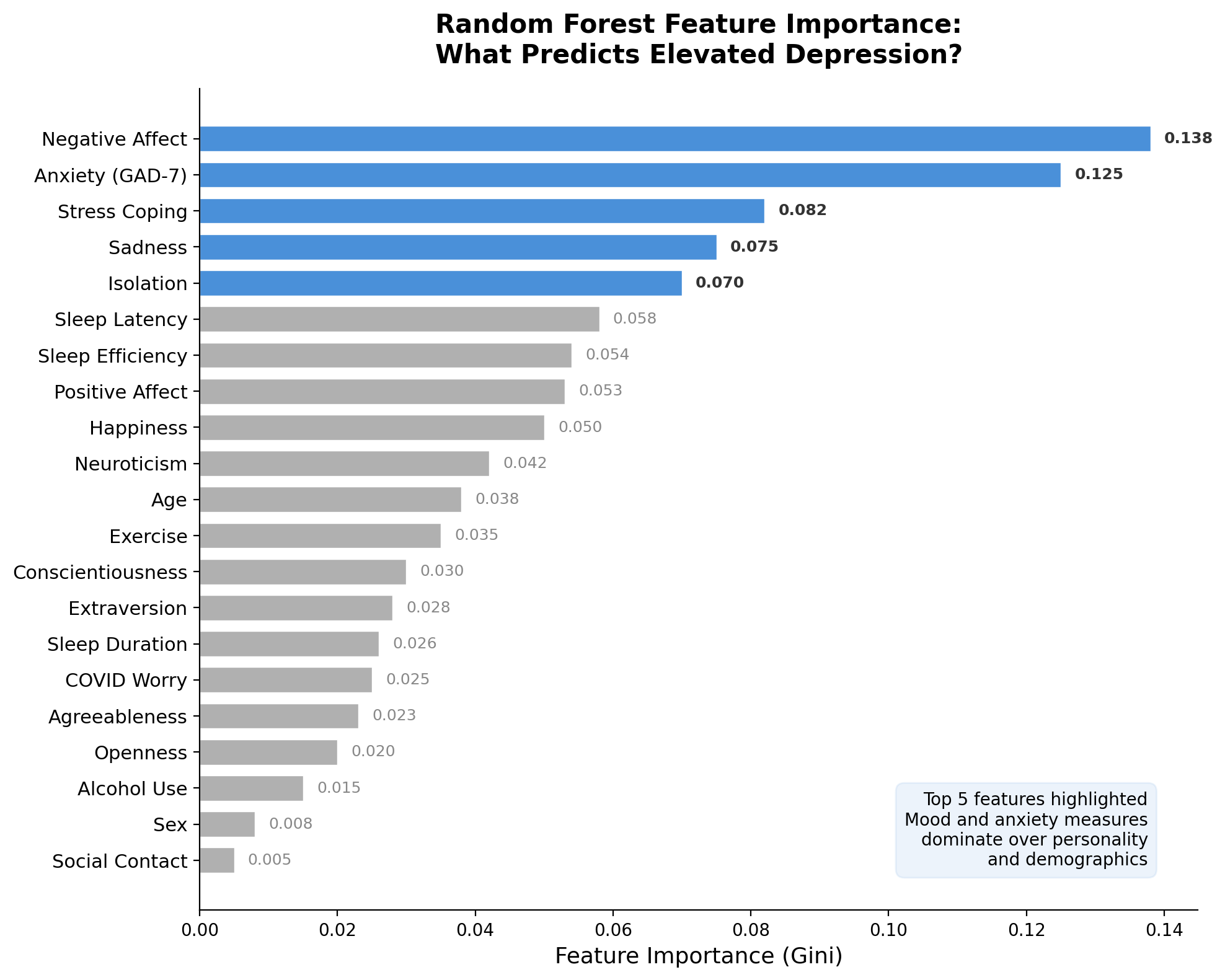
- Mood and anxiety measures dominate — negative affect, GAD-7, stress coping
- Personality and demographics contribute less
- This helps researchers understand what the model relies on — and whether those features make psychological sense
Feature importance can also guide feature selection — drop low-importance features to simplify the model.
Fairness & Ethics
When algorithms affect people
Case Study: COMPAS
COMPAS — Predicting Recidivism in Criminal Justice
An algorithm used in US courts to predict whether defendants would reoffend.
ProPublica found: Black defendants were almost twice as likely to be incorrectly labelled as high risk (false positives) compared to white defendants — even when controlling for prior criminal history.
- Same overall accuracy for both groups
- But different error patterns — same accuracy, different fairness
- This is a classification problem where the type of error matters enormously
Case Study: Healthcare Algorithm Bias
Obermeyer et al. (2019) — Science
A widely-used algorithm identified patients who would benefit from extra care.
The algorithm used healthcare costs as a proxy for health needs. But Black patients historically had less access to healthcare (lower costs) → the algorithm systematically under-identified Black patients who needed care.
The algorithm wasn't “racist” in its code — it learned from biased data that reflected historical inequities.
The Impossibility Theorem
Chouldechova (2017) proved mathematically that when base rates differ between groups, you cannot simultaneously achieve:
Equal false positive rates
across groups
Equal false negative rates
across groups
Equal predictive values
across groups
This isn't a technical problem to solve — it's a values question about which type of fairness matters most in each context.
Common Misconceptions
- “Higher accuracy always means a better model”
- Not when classes are imbalanced. Always check precision, recall, and AUC.
- “Random forests are always better than logistic regression”
- When relationships are roughly linear and data is moderate-sized, logistic regression often matches — and it's more interpretable.
- “The model's output is the final answer”
- The model outputs a probability. Converting to a label requires choosing a threshold — that's a human decision.
- “If the model is accurate, it's fair”
- Overall accuracy can hide very different error rates across groups.
The Classification Pipeline
Same pipeline as regression — different metrics and different model types.
Getting Ready for Week 6
Your second challenge lab
Week 6: Build a Defensible Classifier
- Real data: Boston College COVID-19 Sleep & Well-Being Study
- 836 participants — daily surveys + personality + demographics
- Build and compare four classifiers:
- Baseline → Logistic Regression → Decision Tree → Random Forest
- Target: Elevated depression (PHQ-9 ≥ 5) — nearly balanced (55% / 45%)
- Justify your threshold — why 0.5? Why not 0.3 or 0.7?
- Report proper classification metrics — not just accuracy
New LLM Skill: Refactoring
Week 2: Prompting · Week 4: Debugging · Week 6: Refactoring
Weak prompt
“Clean up my code.”
Strong prompt
“Refactor this pipeline to: (1) separate data loading from modelling, (2) add assertions to verify data shape after each merge, (3) create a reusable function for fitting and evaluating a model, (4) add docstrings, (5) add comments explaining why each step is done. Prioritise readability over cleverness.”
Refactoring = making code cleaner and more maintainable without changing what it does.
Before Next Week
Download the data
conda activate psyc4411-env
cd weeks/week-06-lab/data
python download_data.py
Downloads ~22 MB of CSV files. If you've already done this for a Week 4 bonus challenge, the files will already be there.
Review
- Read the companion reading if you haven't
- Review: confusion matrix, precision, recall, F1, AUC
- Know the difference between a tree and a forest
Key References
- Steyerberg et al. (2010) — Assessing prediction model performance
- Obermeyer et al. (2019) — Dissecting racial bias in healthcare algorithms
- Chouldechova (2017) — Fair prediction with disparate impact
- James et al. (2023) — Intro to Statistical Learning (Python), Ch 4
- statlearning.com — Free PDF
Full reading list: readings.md